Playing with a Rational Distribution

11 Sep 2022

(Note to reader: I think I wrote this post for myself. From an outside perspective, it’s by far the most boring one I’ve ever written. But it’s math that’s been occupying my mind for a week and from an inside perspective it’s been quite fun. Maybe you’ll find the fun in it that I did.)

For a project I’m currently working on at GitHub, I ran into my first statistical distribution defined on rational numbers and I found it weird and interesting when compared to the continuous distributions that I’m used to. We were looking at feature adoption on a per-repository basis. We defined adoption to be

\[\textrm{adoption}=\frac{\textrm{number of people using feature in a given repo}}{\textrm{number of people active in that repo}}\]

The question is, what should the distribution of feature adoption look like across all repos? Pause here and think about it. (Don’t even scroll down!) Leaning upon my normal intuition with continuous distributions I was initially a bit surprised with what I found.

Motivation with an Analogous Continuous Distribution.

Let’s make a ridiculous assumption. Rather than having a distinct integer number of people active in a repo, you can have a real-valued number of people. Yep, you can have 32.74 active users, or \(\pi\) users for that matter. Most likely the distribution would be long tailed with most repos having a relatively low number of users, say 0 to 7.3 users, but a few repos having a large number of users say 1000.2 users. Let’s describe this using the exponential distribution so that \(X\) is the number of people active in that repo.

\[f_X(x;\lambda) = \lambda e^{-\lambda x}\;\;\;\;\;\;(\textrm{for }x >= 0)\]

Then, for each repo, some also real-valued number of users is going to be using the feature. The number of feature users must be less than or equal to the number of users in the repo. For simplicity sake, let’s say that this distribution, \(Y\vert X\), is uniform from 0 to the number of active users.

\[f_{Y|X}(y|x) = 1/x\]

This implies a joint distribution:

\[f_{X,Y}(x,y) = \lambda e^{-\lambda x}/x\]

But we’re interested in adoption, which I’ll label \(R\) because it’s the ratio \(R=Y/X\). We can arrive at \(f_{X,R}\) by substituting in \(y=rx\) and trivially arrive at the same formula since there’s no \(y\) in the equation.

\[f_{X,R}(x,r) = \lambda e^{-\lambda x}/x\]

In order find \(f_R(r)\) we marginalize out the \(X\). This is a bit awkward, because we’re in “ratio” space. So let’s look at what happenes when we marginalize both \(X\) and \(R\) out. In this case, the result is 1, meaning that there’s a 100% chance that \(X\) will take on some value from 0 to \(\infty\) and that \(R\) will take on some value from 0 to 1.

\[\iint\limits_{X,R}f_{X,R}(x,r) \mathrm{d}A = 1\]

The awkward part here is that the differential area in this case is actually \(\mathrm{d}A = x\, \mathrm{d}x\, \mathrm{d}r\). (Do you remember doing funny things in calc class when integrating in cylindrical space… we have to do something like that here.)

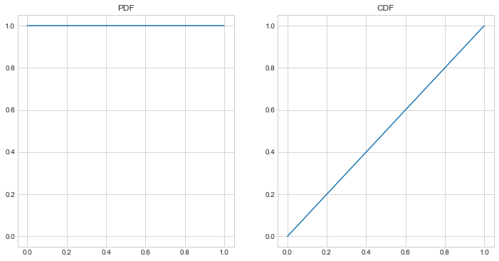
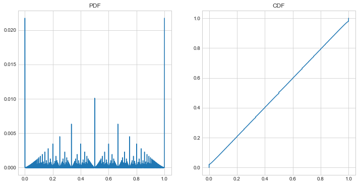
\[\begin{matrix} \iint\limits_{X,R}f_{X,R}(x,r) \mathrm{d}A &=& \int_0^1 \int_0^\infty \frac{\lambda e^{-\lambda x}}{x} x\, \mathrm{d}x\, \mathrm{d}r \\ &=& \int_0^1 \int_0^\infty \lambda e^{-\lambda x} \mathrm{d}x\, \mathrm{d}r \\ &=& \int_0^1 1 \mathrm{d}r \\ &=& \int_0^1 f_{R}(r) \mathrm{d}r \\ &=& 1 \end{matrix}\]

The big point here is that \(f_R(r) = 1\), that is, the distribution of the adoption ratio is just uniform from 0 to 1, no matter the choice of \(\lambda\). And for the purpose of comparison below, here is what the PDF and CDF of the ratio distribution looks like:

Considering the Analogous Discrete Distribution.

We now make more reasonable assumptions about the indivisibility of our users – users are discrete. (Thank goodness. It was getting messy with all the pieces of users from the last section.) The number of people active in a given repo, \(X\), is given by the discrete analog of the exponential distribution, the geometric distribution.

\[f_X(x) = (1-p)^{x-1}p\;\;\;\;\;\;(\textrm{for }x >= 1)\]

Similarly, given the number of people active in a repo, \(x\), the number of them that are using the feature \(y\) is uniformly distributed from 0 to \(x\).

\[f_{Y|X}(y|x) = \frac{1}{x+1}\]

This implies a joint distribution of

\[f_{X,Y}(x,y) = \frac{(1-p)^{x-1}p}{x+1}\]

And as in the continuous example, we’re really interested in the ratio \(R=X/Y\). Now, if you thought that marginalizing the continuous distribution was awkward, check out what we’re going to do with the discrete distribution. First, we’re going to make a table of \(f_{X,Y}\) for all values of \(x\) and \(y\).

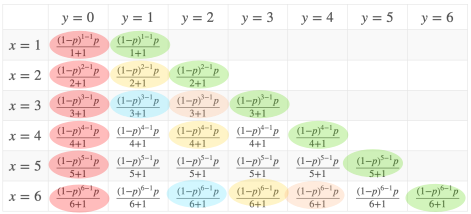
This is this the top left portion of the table. The table extends infinitely towards \(x=\infty\) and \(y=\infty\). Next, as you can see above, we take note of the values where the ratio is the same: red cells where \(r=0\), green where \(r=1\), yellow where \(r=\frac{1}{2}\), blue where \(r=\frac{1}{3}\), orange where \(r=\frac{2}{3}\)… if we keep going, then every cell in the infinite chart will get colorized according to a unique ratio. The probability mass function (PMF) of \(R\) then is just adding up all the cells that correspond to the same ratio. For instance:

\[f_R\left( \frac{1}{2} \right) = \frac{(1-p)^{2-1}p}{2+1} + \frac{(1-p)^{4-1}p}{4+1} + \frac{(1-p)^{6-1}p}{6+1} + \cdots\]

and

\[f_R\left( \frac{2}{3} \right) = \frac{(1-p)^{3-1}p}{3+1} + \frac{(1-p)^{6-1}p}{6+1} + \frac{(1-p)^{9-1}p}{9+1} + \cdots\]

See the pattern? If the lowest common denominator of \(r\) is \(d\), then

\[f_R(r) = \Sigma_{i=1}^\infty \frac{(1-p)^{di-1}p}{di+1}\]

But through much magic we can “simplify” equation. First we introduce a substitution to make the equation a little easier to deal with: \(q=1-p\)

\[\begin{matrix} f_R(r) &=& \Sigma_{i=1}^\infty \frac{q^{di-1}(1-q)}{di+1} \\ &=& (1-q)\Sigma_{i=1}^\infty \frac{q^{di-1}}{di+1} & \textrm{pull common term out of sum} \\ &=& (1-q)\Sigma_{i=1}^\infty \frac{q^{di-1}}{di+1}\frac{q^2}{q^2} & \textrm{multiply by 1 so that...} \\ &=& \frac{1-q}{q^2}\Sigma_{i=1}^\infty \frac{q^{di+1}}{di+1} & \textrm{...the exponent and the denominator are the same} \\ &=& \frac{1-q}{q^2}\Sigma_{i=1}^\infty \int \frac{\mathrm{d}}{\mathrm{d}q} \frac{q^{di+1}}{di+1} \mathrm{d}q & \textrm{introduce integral and derivative}\\ &=& \frac{1-q}{q^2}\Sigma_{i=1}^\infty \int q^{di} \mathrm{d}q & \textrm{take the derivative} \\ &=& \frac{1-q}{q^2}\int \Sigma_{i=1}^\infty q^{di} \mathrm{d}q & \textrm{swap the integral and the summation} \\ &=& \frac{1-q}{q^2}\int \frac{q^d}{1-q^d} \mathrm{d}q & \textrm{rewrite geometric series as fraction}\\ &=& \frac{(1-q)q^{d+1}}{q^2} \frac{_2F_1 \left( 1,1+\frac{1}{d};2+\frac{1}{d};q^d \right)}{d+1} & \textrm{ask WolframAlpha to solve the integral} \\ &=& p(1-p)^{d-1} \frac{_2F_1 \left( 1,1+\frac{1}{d};2+\frac{1}{d};(1-p)^d \right)}{d+1} & \textrm{substitute in }q=1-p\\ \end{matrix}\]

It’s hard to look at that mess and think that it’s simpler. Also we had to introduce the very foreign-looking hypergeometric function \(_2F_1\). But it’s no longer an infinite series! So computing the value is quite a bit faster than attempting to compute enough terms of the infinite series so as to be “close enough”, especially for low values of \(p\). (Still though, it would have made my day if this ended up being a log or something.)

Great, fine, whatever, let’s see the PMF and CMF.

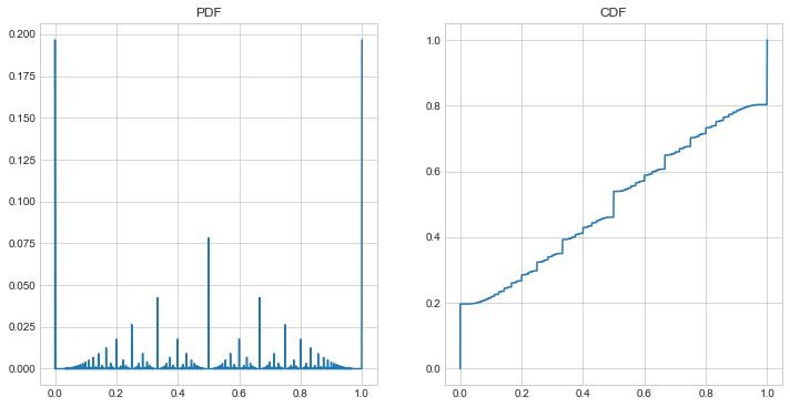
Whoa! For something that I thought was going to be analogous to the uniform distribution in the continuous example above, this is radically different! And it’s kinda cool looking!

But Why?

It’s actually somewhat intuitive that we should see a shape like this once we think for a bit. Since the ratio has integers in both the numerator and the denominator, and since the geometric distribution favors smaller numbers, then you can expect to see a lot more fractions like \(\frac{1}{2}\), and \(\frac{2}{3}\), and \(\frac{1}{4}\), and a lot fewer like \(\frac{27}{624}\). But it’s pretty neat that a distribution over rational numbers with a fractal PMF was just hiding in plain sight. Though really, as I think about it more, I suspect any distribution defined across rational numbers is going to be similarly fractal.

Wait There’s More!

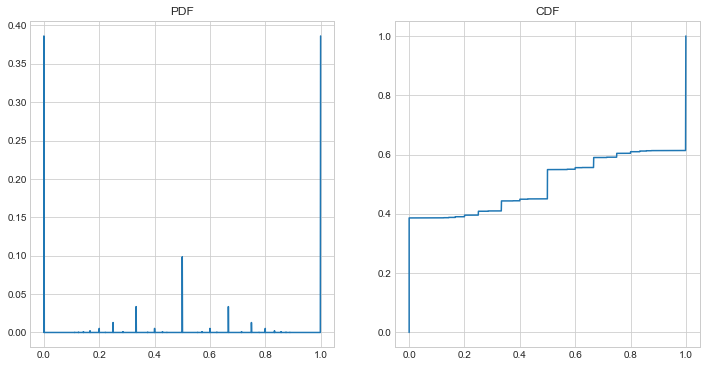
One more thing. As we can see in the CMF above, the distribution is really heavy towards the beginning and end and for big fractions because of the reasons mentioned in the last section. But we can smooth that out by our choice of \(p\) in the geometric distribution. For the above example, \(p=0.125\). If we make \(p\) higher, say \(p=0.5\), then it further favors smaller integers and the graph gets spikier.

And as \(p\) approaches 0:

(here \(p=0.005\)), the CMF approaches uniformity. However the PMF looks wilder, and more fractal than ever. The shape of the plot appears to be converging to the same shape as a Farey Diagram, but at the same time, the absolute height of each value is approaching 0. And maybe that’s a good note to end this post on… what does it mean to have a function defined on rationals that has a definite shape (in terms of the ratios of the values of \(f_R\)), but has infinitesimal values? Weird, right?

Special thanks

Thanks to Meijke Balay and Jason Orendorff for some of the tips and tricks above, Meijke Balay for pointing me to the Farey sequence, and Taj Singh for helping make my LaTeX prettier.