"Who da Boss" Graph Clustering
07 Aug 2022I’ve been playing with my Twitter social graph recently, and it occurred to me that the people that I’m friends with form several clusters. I wanted to see if I could come up with some sort of clustering algorithm to identify these clusters. Why? Well for one, it could be of practical use; maybe I can find some good use for it. But, perhaps more than that, I was curious if I could make a clustering algorithm – I’ve kinda got a thing for reinventing wheels.
The Algorithm
Consider the following graph. There are two obvious clusters here, the 5 nodes on the left including node 2 at their center and the 4 nodes on the right including node 7 at their center.
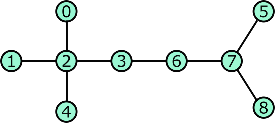
Let’s pretend that each node is a person. As a group, they wish to somehow fairly elect the leaders of the graph. There will be multiple leaders, one leader per cluster. How can they communicate information with their neighbors and arrive at a fair and agreed upon choice for leaders of ths graph?
Here is how they proceed:
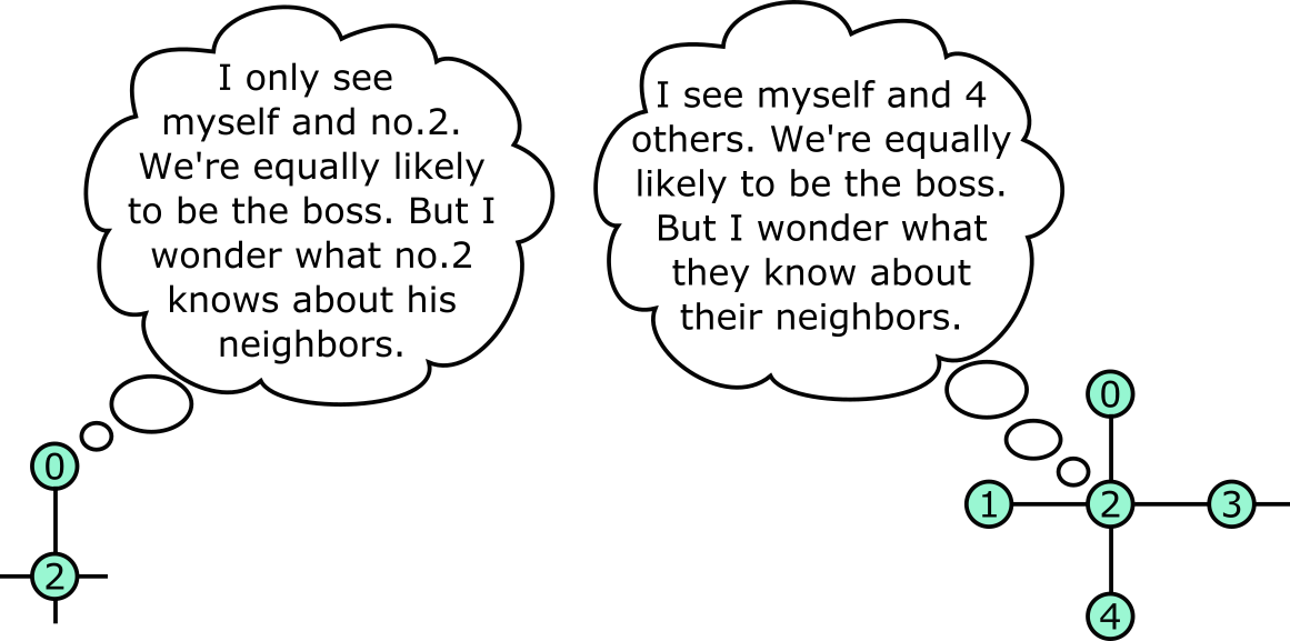
Step 1: Each node looks around and takes a first estimate of “who’s the boss” by assuming that themself or their immediate neighbors are equally likely to be the boss. So, for instance node 0 assumes there’s a 50% chance that they are the boss and a 50% chance that node 2 is their boss. Similarly, node 2 assumes that there is a 20% that they are the boss and a 20% chance for each of nodes 0, 1, 3, and 4.
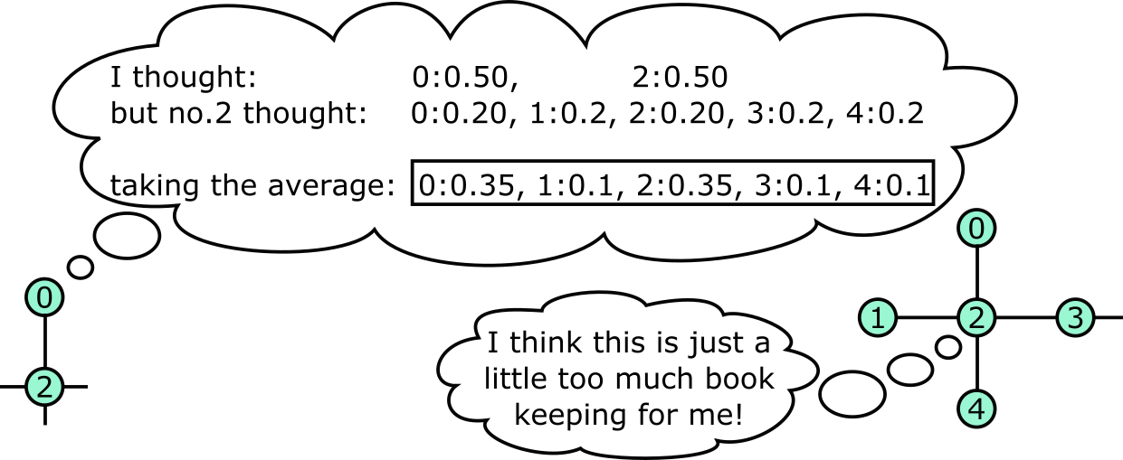
Step 2: Each node confers with its neighbors. It creates a weighted average of the a priori distributions of itself and all of it’s neighbors. (The weights are the values of each node’s own priori distribution.)
Step 3: The distribution is “exaggerated”, so that the high probabilities are made higher and the lower probabilities are made lower. For instance, if the values of the distribution are labeled \(d_i\), then the exaggerated values are \(\hat{d}_i=d_i^g / \Sigma_j d_j^g\) where \(g\) is the “granularity”. A higher granularity will result in more, smaller clusters.
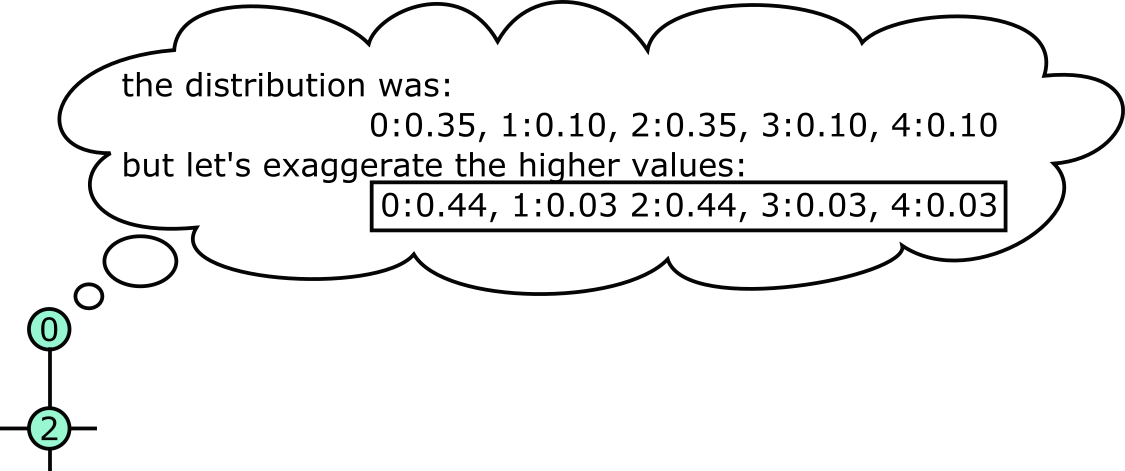
This is an important step! If we didn’t exaggerate the high-scoring nodes and diminish the low-scoring nodes, then the distributions would never converge to a single winner.
Step 4: Finally, we go back to Step 2 and keep iterating until each node has clearly decided which node will be its leader – namely, the distribution will be ~1.0 for a single node ~0.0 for all the others.
Better Bookkeeping with Matrices
Each node has a lot to keep up with, and writing for-loops and data arrays to keep up with this stuff would be a nightmare. Fortunately matrix algebra serves as a great medium for tracking all of these numbers and implementing the algorithm above. So, let’s work the same example problem again, but this time with matrices!
The first thing we do is create the adjacency matrix that represents the above graph. And adjacency matrix has rows and columns that correspond the nodes in the graph. Everywhere that the matrix has a value of 1, that indicates that the node corresponding to that row is connected to the node corresponding to that column. Here is how we create an adjacency matrix for the example graph above.
connections = [
    (0,2),
    (1,2),
    (2,3),
    (2,4),
    (3,6),
    (5,7),
    (6,7),
    (7,8),
]

n = 9
rows, cols = list(zip(*connections))
A = np.zeros([n,n])
A[rows,cols] = 1
A[cols,rows] = 1
A = A + np.identity(A.shape[0])
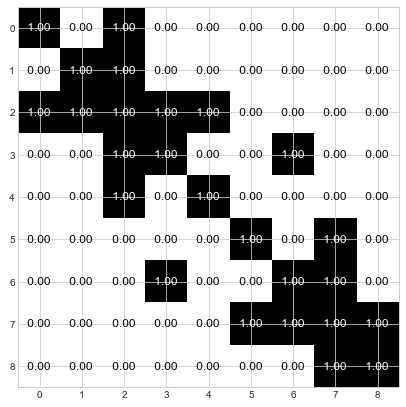
Below is our adjacency matrix printed as an image. The top row, shows that node 0 is connected to itself and to node 2. Row 2 shows that node 2 is connected to itself and to nodes 0, 1, 3, and 4. Check for yourself that the adjacencies are correct. Now we’re ready to begin.
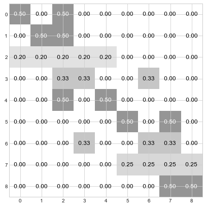
Step 1: Determine the a priori distribution by normalizing each row to sum to 1.0.
D = A/np.sum(A, axis=1, keepdims=True)
Step 2: Confer with neighboring nodes and create a weighted average of their distributions. With matrices, this step works out beautifully - it’s just a matrix multiplication.
D = D @ D
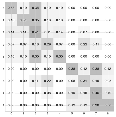
Compare the values in row 0 with node 0’s step 2 statement in the cartoon above. Samezies!
Step 3: Exaggerate the more likely candidates and diminish the less likely candidates.
pow_D = np.power(D, granularity)
sum_pow_D = np.sum(pow_D, axis=1, keepdims=True)
D = pow_D / sum_pow_D
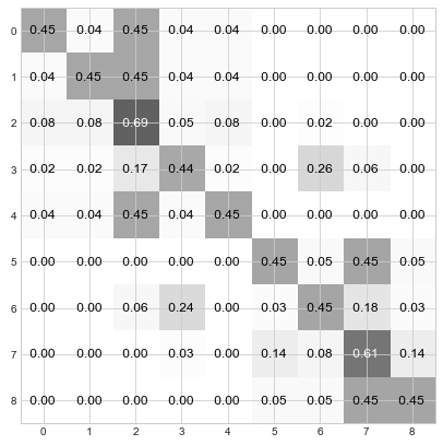
Compare the values in row 0 with node 0’s step 3 statement in the cartoon above. Samezies! Er… well Python rounded differently than me, but you get the point.
Step 4: Keep iterating through steps 2 and 3 until the distributions converge. For the current example, this is done in about 3 more steps:
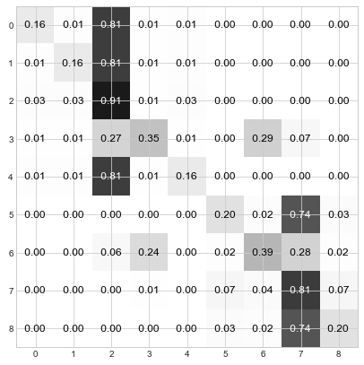
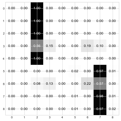
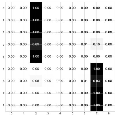
Et voila! You can see that the nodes have used the “Who da Boss” protocol to elect 2 leaders. Nodes 0, 1, 2, 3, and 4 have elected node 2 as their leader and Nodes 5, 6, 7, and 8 have elected node 7 as their leader. And if you refer back to the original graph, this division of leadership seems quite reasonable – there are two main groups, and node 2 is the center of one and node 7 is the center of the other.
Completely assembled, the Who da Boss algorithm is really short and sweet:
import numpy as np

def who_da_boss_dense(A, granularity=2):
    D = A.copy() + np.identity(A.shape[0])
    D = D/np.sum(D, axis=1, keepdims=True)  # Step 1

    # add a tiny amount of noise to the matrix as a tie breaker
    D = D * np.random.uniform(1.0, 1.01, D.shape)

    for i in range(20):
        D = D @ D  # Step 2

        pow_D = np.power(D, granularity)
        sum_pow_D = np.sum(pow_D, axis=1, keepdims=True)
        D = pow_D / sum_pow_D  # Step 3

        if np.all(np.sum(D > 0.99, axis=1) == 1):
            break  # Step 4

    D = (D > 0.99) * 1  # tidy up
    return D
But Will it Work with Real Data?
Well duh. It’d be a pretty lame blog post to make all these pretty images and algorithms and only then figure out that it didn’t actually work. So let’s see it work!
On Twitter I’m JnBrymn. As of this moment, I follow 299 people and 2,132 people follow me. Of all those people I follow, exactly 144 follow me back. These are those people:
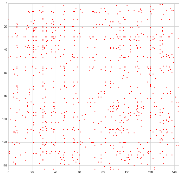
More specifically, this is the adjacency matrix for these users, just like the much smaller one I introduced in the previous section. By looking at the adjacency matrix as-is, it is impossible to discern a pattern of any kind. But let’s apply Who da Boss and then reorganize the rows and columns of this matrix so that people with the same “leader” occupy adjacent rows/columns.

These groupings certainly seem to valid. Look how densely the diagonal block matrices are populated as compared with the off-diagonal block matrices. This means that individuals with the same leader are much more likely to be connected to one-another than they are to people in other groups.
So at a superficial level, at least, the algorithm seems to work. But let’s go a level deeper. I can collect the description strings and location strings for every user in each of the sub-groups and then, using MarcelloPerathoner’s suffix-tree library, I can extract the common sub-strings in order to see what each group is about. Here’s how that plays out for the larger groups:
| no. | description strings | location strings | commentary |
|---|---|---|---|
| 1 | ‘charlottesville’, ‘entrepreneur’, ‘founder’, ‘search’ | ‘charlottesville, va’ | When I lived in Cville I was very connected to the entrepreneourship and search tech communities |
| 2 | ‘@eventbrite’ | ‘san francisco, ca’, ‘nashville, tn’ | I was formerly employed at Eventbrite, a company based in SF and Nashville |
| 3 | ‘opinions are’, ‘@github’ | (none) | I am currently employed ay GitHub, an internationally distributed company (thus no location listed) |
| 4 | ‘data scien’, ‘engineer’ | ‘nashville, tn’ | After moving to Nashville I connected with the software and data science communities. |
| 5 | ‘python’ | (none) | Who doesn’t like Python? I know I do! |
So not bad, right? I think with a little massaging, the Charlottesville entrepreneur community in group 1 could have been disentangled from my Charlottesville search technology friends. But then again, Charlottesville was a pretty tight-knit community.
Now what?
We could go in plenty of directions from here.
For one, I wish the theory behind this algorithm was a little more mature. While I hope you’ll agree that it makes intuitive sense, I should like to be able to highlight certain criteria for a good grouping algorithm and show that Who da Boss ensures this criteria is met. For instance “local consensus”: I would like to show that a neighborhood of users will always elect a single leader rather than a mixture of leaders. Similarly, I would like to figure out how to optimize the granularity parameter so that we strike a balance between maximizing the number of clusters while minimizing out-of-cluster connections.
Perhaps the algorithm can be applied to clustering outside of graphs. For instance, rather than starting with a sparse adjacency matrix, the math would work all the same if we started with a dense pairwise similarity matrix. I’ve actually attempted this using Scikit Learn’s 20Newsgroups dataset. But since the new article titles were very short, the clustering was noisy and not terribly accurate. Perhaps it would work better with longer pieces of text.
Another interesting possibility is to sparsify the algorithm. Step 3 above diminishes the less important connections values for each node. We could instead just set these values to 0 and thereby keep the distribution matrix sparse. If the algorithm retained sparse matrices throughout, then it would be amenable to clustering much larger graphs.