EARRRL – the Estimated Average Recent Request Rate Limiter - the Mathy Bits
18 Mar 2021In the companion post I introduced a problem with naive, window-based rate limiters – they’re too forgiving! The user’s request count is stored in a key in Redis with a TTL of, say, 15 minutes, and once the key expires, the abusive user can come back and immediately offend again. Effectively the abusive user is using your infrastructure to rate limit their requests.
In this post we’ll investigate an alternative approach to windowed rate limiting which keeps a running estimate of each user’s request rate and rejects requests for users whose rate is above the prescribed threshold. The focus of this post is on the math behind the approach. For a practical implementation, usage, and motivation for why the math might be worth looking at, please take a look at the companion post.
Not Quite Solving the Problem with Exponentially Weighted Moving Average
The Exponentially Weighted Moving Average is a simple method for measuring the recent average of a series of numbers. (Here’s a great reference.) This makes EWMA seem like a good candidate for building the type of rate limiter described above. Effectively, it would work like this: For each user, you store 2 values, the number of hits in this window and the “running average” of their recent windows. Whenever a user makes a request, you update hit count. At the end of the time window you use a simple formula to incorporate the number of hits into the average of the recent windows, and you also reset the hit count to 0 in preparation for the next window. With this approach, requests would be rejected if the running average of recent requests per window exceeded some prescribed threshold.
Unfortunately, this would-be approach comes with a fatal flaw: you have to perform a calculation for every recently active user at the end of every window. For instance, even if the user did not submit any requests in this time window, you still have to incorporate 0 into their running average, or the running average will never decrease. We’ll have to find some other approach.
Introducing EARRRL
Drawing inspiration from the EWMA, th remainder of this post introduces EARRRL, the Estimated Average Recent Request Rate Limiter. EARRRL limits a user’s requests based upon an estimate of the user’s recent request rate. Importantly, EARRRL requires no global value updates as in the case of EWMA, and EARRRL is not window based, so it doesn’t have the over-permissive forgiveness policy that we see in windowed rate limiters.
Disclaimer: Does this already exist? Eh, probably. It’s just too simple and useful of an idea to not exist. But I couldn’t find it. And after searching the internet for a bit I decided not to find it, because what fun would it be to just look up the answer?!
Theoretical Background
With EARRRL, we wish to estimate the recent average rate at which a user’s requests arrive. Let’s represent the time history of the user’s request rate as \(r(t)\). For the current discussion, time \(t\) is relative to now, so that \(t=0\) means this moment, and \(t=-1\) means one second in the past. In order to take the average, we make use of a weight function, represented as \(w(t)\), which is used to weight the more recent rate as being more important than the rate that occurred further in the past. In order to find the weighted average of the rate, we have to evaluate this integral.
\[\int_{-\infty}^{0} w(t) \cdot r(t)\:dt \tag{1}\](This is very similar to finding the expected value of a function in statistics.)
As of yet, this equation is pretty vague. We can choose the weight function to be whatever we want, and the rate function is dependant upon the user’s behavior, but for both of these, we can make some assumptions that will simplify our work. Let’s start with \(w(t)\). One convenient weighting function is the exponential function:
\[w(t) = \lambda e^{\lambda t} \tag{2}\]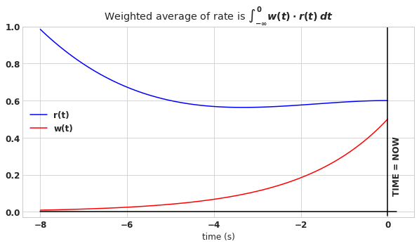
The integral of \(w(t)\) is 1 (a requirement that any weight function must satisfy), and since we will choose \(\lambda\) to be greater than 0, the weight function is fat near to current time and becomes exponentially thinner as we move back in time – thus more recent time is weighted more heavily. (This was our goal, remember.)
In order to gain intuition, let’s look at the recent average of a very simple rate function - a constant rate.
\[\begin{matrix} \int_{-\infty}^{0} w(t) \cdot r(t)\:dt &=& \int_{-\infty}^{0} w(t) \cdot r\:dt \\ &=& r \int_{-\infty}^{0} w(t) \:dt \\ &=& r \\ \end{matrix} \tag{3}\]For the last step, since the integral of a weight function is by definition 1, all that is left is \(r\). This should be a satisfying result, because, if the user’s request rate is constant, \(r\), then the recent average of the rate should just be \(r\), and it is.
If you’re reading carefully, you might notice something weird about the rate function - it’s continuous. What does it mean to have a rate of 0.6 requests per second? You can’t make partial requests. Even though this feels non-intuitive, dealing with a continuous rate is a generalization of the more realistic scenario where requests come in as discrete units. To demonstrate this, we need to introduce the notion of an “impulse” (otherwise known as the Dirac delta). An impulse is the application of an infinitely high rate for an infinitesimally short period of time. However the integral of impulse is finite. Whenever you make a single request, what you’re doing is creating an impulse in the request rate. In an instant, the request rate goes infinitely high because it didn’t take you a second to submit that request (which would be 1 request per second), it didn’t take you a millisecond (which would be 1000 requests per second), it took the twinkling of an eye (which is one request per twinkling). But once that moment passed, the actual number of requests that you made (the integral of the rate) was just 1. (Ok, so that concept is a little difficult to justify in a single paragraph. Look me up on Twitter and I’ll set up a time to explain it more clearly.)
An impulse of size \(N\) (meaning N simultaneous requests in this case) and at some time \(T\) is represented by the notation \(N\delta(t-T)\). And the exponentially weighted average (EWA) of this impulse function is
\[\int_{-\infty}^{0}w(t) \cdot N\delta(t-T)= N \cdot w(T) = N\lambda e^{\lambda T} \tag{4}\](Integration of an impulse is explained in more detail here.) If the time of the impulse is now, \(T=0\), then you can simplify this even more to just \(N\lambda\). Finally, impulses add linearly, so the EWA for \(N_1\) requests occurring at \(T_1\) and \(N_2\) requests occurring at \(T_2\) is \(N_1\lambda e^{\lambda T_1} + N_2\lambda e^{\lambda T_2}\).
The last and most important thing to notice is that there are many possible rate functions that can lead to the same exponentially weighted average value. For example, let’s say that \(\lambda = 0.07\), then a request that just arrived (e.g. and impulse of size \(N=1\) at time \(T=0\)) would have the same EWA as the continuous application of 0.07 requests per second, \(r=0.07\). This would also have the same EWA as two request occurring simultaneously 9.9 seconds ago.
| scenario | equation | avg value |
|---|---|---|
| EWA of one request occuring just now | \(1 \cdot \lambda\) | 0.07 |
| EWA of a constant request rate | \(r\) | 0.07 |
| EWA of 2 requests occuring 9.9 seconds ago | \(2\cdot \lambda e^{-9.9\lambda}\) | 0.07 |
The observation that several different rate time histories correspond to identical EWA values is the crux of the algorithm that we lay out next.
The Algorithm
We now have all the theoretical pieces required to build EARRRL. Our algorithm requires us to track 2 values, the time of the last update \(T\), and the “impulse size” \(N\), which roughly corresponds to the number of recent requests. There are 4 methods for our rate limiter initialize, update, evaluate, and is_rate_limited. They are described here:
Initialize
Upon a user’s first request, set \(T_0=\text{unix_timestamp_now()}\), indicating when the request was made and \(N_0=1\) indicating that it was a single request.
Update
For subsequent requests, \(T_{i-1}\) represents the time of the last request, and \(N_{i-1}\) represents the number of requests were assumed to come at that moment. As in the examples at the end of the last section, we calculate the EWA of \(N_{i-1}\) request happening at \(T_{i-1}\) plus 1 request (the new one) happening right now at \(t=0\). Given this new EWA, we can find an \(N_i\) such that \(N_i\) requests happening at \(t=0\) has an identical EWA value:
| scenario | equation |
|---|---|
| EWA of \(N_{i-1}\) requests at \(T_{i-1}\) and 1 more just now (eq. 4) | \(N_{i-1}\cdot \lambda e^{-\lambda(now-T_{i-1})} + 1 \cdot \lambda\) |
| EWA of \(N_{i}\) requests just now (eq. 4) | \(N_{i}\cdot \lambda\) |
Setting both of these equations equal and solving for \(N_i\) we arrive at \(N\)’s update equation.
\[N_i = 1 + N_{i-1} e^{-\lambda(now-T_{i-1})} \tag{5}\]We also update the time as \(T_i=\text{unix_timestamp_now()}\).
Evaluate
Take a moment and note what we’re doing here. Despite what we said in the update section, it is not true that \(N_i\) requests came at time \(T_i\). However assuming that this is true leads to a relatively good estimate for the recent average rate. This is exactly the quantity we calculate now. Effectively the evaluation step converts from the assumption that all request happened instantaneously at \(T_i\) to the assuption that requests occurred at a constant rate.
Here are the relevant scenarios:
| scenario | equation |
|---|---|
| EWA of \(N_{i}\) requests at \(T_{i}\) (eq. 4) | \(N_{i}\cdot \lambda e^{-\lambda(now-T_{i-1})}\) |
| EWA of a constant request rate (eq. 3) | \(r\) |
Equating these two scenarios, we solve for the assumed constant request rate.
\[r = N_{i}\cdot \lambda e^{-\lambda(now-T_{i-1})} \tag{6}\]This is the important number! It’s the estimated average recent request rate – it’s what we are limiting.
Is Rate Limited
Finally we introduce the actual rate limiting policy: If the estimated average recent request rate is higher than the maximum allowed request rate, then is_rate_limited returns true, otherwise false.
In Code
The end result in Python is refreshingly simple:
class EARRRL:
    def __init__(self, lambd, rate_limit):
        self.N = 1
        self.T = time.time()
        self.lambd = lambd
        self.rate_limit = rate_limit

    def update(self):
        delta_t = self.T - time.time()
        self.N = 1 + self.N*math.exp(self.lambd*delta_t)
        self.T = time.time()

    def evaluate(self):
        delta_t = self.T - time.time()
        return self.N*self.lambd*math.exp(self.lambd*delta_t)

    def is_rate_limited(self):
        return self.evaluate() > self.rate_limit
(See the companion post for practical examples of implementing and using this in Redis.)
Does it Really Work?
Everything above is based on intuition. Now let’s toss together some light proofs to indicate that this algorithm performs as advertised.
Asymptotic Convergence for Constant (Discrete) Request Rate
If a user consistently makes a request every \(\Delta t\) seconds, then we would like EARRRL to converge to the correct estimate of the request rate \(r = \frac{1}{\Delta t}\). To investigate this, let’s watch as the \(N\) value of the algorithm is updated (ref eq. 5).
| time | N equals | N equals (rearranged) |
|---|---|---|
| \(0\) | \(0\) | \(0\) |
| \(\Delta t\) | \(1\) | \(1\) |
| \(2\Delta t\) | \(1 + e^{-\lambda \Delta t}\) | \(1 + e^{-\lambda \Delta t}\) |
| \(3\Delta t\) | \(1 + (1 + e^{-\lambda \Delta t})e^{-\lambda \Delta t}\) | \(1 + e^{-\lambda \Delta t} + e^{-2\lambda \Delta t}\) |
| \(4\Delta t\) | \(1 + (1 + e^{-\lambda \Delta t} + e^{-2\lambda \Delta t})e^{-\lambda \Delta t}\) | \(1 + e^{-\lambda \Delta t} + e^{-2\lambda \Delta t} + e^{-3\lambda \Delta t}\) |
And as time progresses, \(N\) converges to
\[N \rightarrow 1 + e^{-\lambda \Delta t} + e^{-2\lambda \Delta t} + e^{-3\lambda \Delta t} \cdots = \sum_{k=0}^{\infty}e^{-k\lambda \Delta t} \tag{7}\]Already we see a nice result: Applying eq. 4, to eq. 7 we see that the exponentially weighted average of \(N\) simultaneous requests that occurred just now is equivalent to the to the EWA of a series of requests spaced \(\Delta t\) seconds apart. Thus, EARRRL is accurately tracking the exact EWA rate in this case rather than some approximation.
Further, note that Eq. 7 is a geometric series which converges to
\[N \rightarrow \sum_{k=0}^{\infty}e^{-k\lambda \Delta t} = \frac{1}{1-e^{-\lambda \Delta t}} \tag{8}\]From this equation, we multiply by \(\lambda\) to get the EWA of the request rate at the moment just after a request is received.
\[\text{EWA of rate upon arrival of request} = \frac{\lambda}{1-e^{-\lambda \Delta t}} \tag{9}\]And if we multiply eq. 7 by \(\lambda e^{-\lambda \Delta t}\) we get the EWA of the request rate \(\Delta t\) later, just before the next request is received.
\[\text{EWA of rate just before arrival of next request} = \frac{\lambda e^{-\lambda \Delta t}}{1-e^{-\lambda \Delta t}} \tag{10}\]Note that neither of these values is the true rate \(r=\frac{1}{\Delta t}\), rather referring to the plots in the companion post, these are the values that EARRRL bounces between when subject to a constant rate of requests. Notice that when you subtract the two equations, the result is simply \(\lambda\). Thus, the smaller that you make \(\lambda\) the more accurate EARRRL will become.
Take another look at both equations 9 and 10, as \(\lambda\) approaches zero, these equations approach the same value and at the limit this value indeed equals the true request rate. This can be shown with help from l’Hopital’s rule. For example, starting from eq. 9:
\[r = \lim_{\lambda \rightarrow 0} \frac{\lambda}{1-e^{-\lambda \Delta t}} = \lim_{\lambda \rightarrow 0} \frac{\frac{d}{d\lambda}\lambda}{\frac{d}{d\lambda}(1-e^{-\lambda \Delta t})} = \lim_{\lambda \rightarrow 0} \frac{1}{\Delta t e^{-\lambda \Delta t}} = \frac{1}{\Delta t}\]Thus as \(\lambda\) approaches zero, the estimated rate of a sequence of evenly spaced requests does indeed converge to the correct value \(r = \frac{1}{\Delta t}\).
Choosing Lambda to Control Response Time and Accuracy Tradeoff
We saw above (just past eq. 9 and 10) that \(\lambda\) controls the accuracy of EARRRL, but it also controls how fast EARRRL converges. To see this, take a look at the evaluation function (eq. 6) restated here
\[r = N_{i} \lambda e^{-\lambda(\Delta T_i)}\]At the moment just after the last request occurred, the EWA of rate was \(r=N_{i} \lambda\), so let’s define the half-life \(T_{\lambda}\) as the amount of time that it take for the estimate to drop by half assuming no new requests come in. In other words, let’s solve this equation for \(T_{\lambda}\):
\[N_{i} \lambda e^{-\lambda(T_{\lambda})} = \frac{N_{i} \lambda}{2} \tag{11}\]The answer is:
\[T_{\lambda} = \frac{\ln 2}{\lambda} \tag{12}\]The half-life is inversely proportional to \(\lambda\). Therefore requiring twice the accuracy implies a response time that is twice as slow. However it is our good fortune that we don’t care much about response time. As a matter of fact, it is probably better to have a slow response time so that EARRRL doesn’t prematurely rate limit a user upon receiving a small burst of queries (see next section). Instead, EARRRL is designed to protect against the users that consistently exceed the prescribed rate limit.
Burst Saturation and Attempting to Game the System
We’ve demonstrated that if a user makes periodic requests at a consistent rate, that EARRRL will converge to an accurate estimate of their rate. But what happens if the user’s behavior is bursty rather than consistent? Let’s consider the worst case scenario: how many requests can a user make instantaneously before EARRRL saturates? According the evaluation equation (eq. 6), this number is:
\[N_{\text{saturation}}=\frac{r_{\text{threshold}}}{\lambda} \tag{13}\]Since you are in control of \(\lambda\), it’s a good idea to make sure that \(N_{\text{saturation}}\) is quite high, because if it really is just a small burst, you don’t necessarily want to penalize the user.
Now this begs a question: Can a user game the system by bursting up to the saturation threshold, then waiting for a cool down period and then bursting again? The goal, of course, would be to sneak past the rate limit. Let’s see what happens in this scenario. Let’s say the user sends \(N_{\text{saturation}}\) requests and then waits several half-lives until the rate estimate is back near to 0. Let’s pick 5 half-lives (97% of the way back to 0). In this case the user’s overall send rate is \(r_{\text{abuse}}=\frac{N_{\text{saturation}}}{5T_{\lambda}}\). Plugging in eq. 12 and 13:
\[r_{\text{abuse}}= \frac{N_{\text{saturation}}}{5T_{\lambda}} = \frac{r_{\text{threshold}}}{\lambda} \frac{\lambda}{5\ln 2} = \frac{r_{\text{threshold}}}{5\ln 2} \tag{14}\]Since \(5\ln 2\) is so much larger than 1, then the abuse rate is going be well below the EARRRL threshold and we are safe from anyone gaming the system in this manner.
Conclusion
EARRRL, the Estimated Average Recent Request Rate Limiter provides an appealing alternative to the standard, windowed rate limiter. It is intuitive to use, you just specify a threshold for the rate and a value for \(\lambda\) to bound the error. The benefit of EARRRL is that it automatically “permanently bans” users who are willing to consistently abuse rate limits, but at the same time, it is forgiving of users, even formerly abusive users, who have demonstrated that they will maintain a rate limit below the prescribed threshold. EARRRL also allows for occasional bursty behavior for which windowed rate limiters might prematurely rate limit good users.
What’s next?
- Want to go build one? Check out the companion post where I create a simple Redis implementation.
- Want to play with the algorithms yourself? Check our my Jupyter notebook
- What tell me what you think? Look me up.